SQL Server POLYVAL Function
Updated 2024-03-06 21:33:04.597000
Description
Use the aggregate function POLYVAL for calculating a new y-value given a new x-value using the coefficients of a polynomial p(x) of degree n that fits the x- and y-values supplied to the function. The y-value is calculated using n+1 polynomial coefficients in descending powers:
y=p_1x^n+p_2x^{n-1}+\dots+p_nx^1+p_{n+1}x^0
Syntax
SELECT [wct].[POLYVAL] (<@known_x, float,>
<@known_y, float,>
<@degree, smallint,>
<@new_x, float,>)
Arguments
@known_y
the y-values to be used in the calculation. @known_y must be of the type float or of a type that implicitly converts to float.
@degree
an integer specifying the degree of the polynomial.
@new_x
the new x-value for which you want POLYVAL to calculate the y-value.
Return Type
float
Remarks
The x- and y-values are passed to the function as pairs.
If x is NULL or y is NULL, the pair is not used in the calculation.
Use the POLYFIT or POLYFIT_q functions to get the coefficients.
@degree must remain invariant for the GROUP.
@new_x must remain invariant for the GROUP.
Examples
In this example, we will use the SeriesFloat function to generate a series of x-values equally spaced in the interval [0, 2.5] and then evaluate the error function, ERF, at those points. We will specify an approximating polynomial of 6 degrees. We will then generate values at the midpoint for each interval using the approximating polynomial.
SET NOCOUNT ON;
SELECT SeriesValue as x,
       westclintech.wct.ERF(SeriesValue) as y
INTO #erf
FROM wct.SeriesFloat(0, 2.5, 0.1, NULL, NULL);
SELECT a.seriesvalue as x,
       wct.POLYVAL(e.x, e.y, 6, seriesvalue) as POLYVAL
FROM wct.SERIESFLOAT(0.05, 2.5, 0.1, NULL, NULL) a ,
     #erf E
GROUP BY seriesvalue;
DROP TABLE #erf;
This produces the following result.
| x | POLYVAL |
|---|---|
| 0.05 | 0.0560409087420763 |
| 0.15 | 0.167414870029564 |
| 0.25 | 0.276183548384518 |
| 0.35 | 0.379669434495585 |
| 0.45 | 0.475932241043269 |
| 0.55 | 0.563669129052707 |
| 0.65 | 0.642120996194105 |
| 0.75 | 0.710984827030842 |
| 0.85 | 0.770332105215247 |
| 0.95 | 0.82053328763204 |
| 1.05 | 0.862188340489436 |
| 1.15 | 0.896063337357925 |
| 1.25 | 0.923033119156717 |
| 1.35 | 0.944030016087848 |
| 1.45 | 0.959998631517963 |
| 1.55 | 0.971856687807761 |
| 1.65 | 0.980461934089109 |
| 1.75 | 0.986585115989822 |
| 1.85 | 0.990889007306113 |
| 1.95 | 0.993913503622709 |
| 2.05 | 0.996066777880637 |
| 2.15 | 0.997622497892672 |
| 2.25 | 0.998723105806456 |
| 2.35 | 0.999389159515293 |
| 2.45 | 0.999534736016589 |
Since we know that the y-values are actually erf(x), in this example we will compare the values calculated using the approximating polynomial and erf(x).
SET NOCOUNT ON;
SELECT SeriesValue as x,
       westclintech.wct.ERF(SeriesValue) as y
INTO #erf
FROM wct.SeriesFloat(0, 2.5, 0.1, NULL, NULL);
SELECT x,
       POLYVAL,
       [ERF(x)],
       POLYVAL - [ERF(x)] as [DIFFERENCE]
FROM
(
    SELECT a.seriesvalue as x,
           wct.POLYVAL(e.x, e.y, 6, a.seriesvalue) as POLYVAL,
           westclintech.wct.ERF(a.SeriesValue) as [ERF(x)]
    FROM wct.SERIESFLOAT(0.05, 2.5, 0.1, NULL, NULL) a ,
         #erf E
    GROUP BY seriesvalue
) m;
DROP TABLE #erf;
This produces the following result.
| x | POLYVAL | ERF(x) | DIFFERENCE |
|---|---|---|---|
| 0.05 | 0.0560409087420763 | 0.0563719777970165 | -0.00033106905494016 |
| 0.15 | 0.167414870029564 | 0.167995971427363 | -0.000581101397799128 |
| 0.25 | 0.276183548384518 | 0.276326390168236 | -0.000142841783717984 |
| 0.35 | 0.379669434495585 | 0.379382053562309 | 0.00028738093327535 |
| 0.45 | 0.475932241043269 | 0.475481719786923 | 0.000450521256346315 |
| 0.55 | 0.563669129052707 | 0.563323366325108 | 0.000345762727599452 |
| 0.65 | 0.642120996194105 | 0.642029327355671 | 9.16688384339226E-05 |
| 0.75 | 0.710984827030842 | 0.711155633653513 | -0.000170806622671549 |
| 0.85 | 0.770332105215247 | 0.770668057608351 | -0.000335952393103467 |
| 0.95 | 0.82053328763204 | 0.820890807273276 | -0.000357519641236315 |
| 1.05 | 0.862188340489436 | 0.862436106090095 | -0.000247765600658978 |
| 1.15 | 0.896063337357925 | 0.896123842936913 | -6.05055789882902E-05 |
| 1.25 | 0.923033119156717 | 0.922900128256456 | 0.000132990900260643 |
| 1.35 | 0.944030016087848 | 0.943762196122722 | 0.000267819965126148 |
| 1.45 | 0.959998631517963 | 0.959695025637457 | 0.000303605880506042 |
| 1.55 | 0.971856687807761 | 0.97162273326201 | 0.000233954545751147 |
| 1.65 | 0.980461934089109 | 0.980375585023358 | 8.63490657508903E-05 |
| 1.75 | 0.986585115989822 | 0.98667167121918 | -8.65552293580762E-05 |
| 1.85 | 0.990889007306113 | 0.991111030056084 | -0.000222022749971074 |
| 1.95 | 0.993913503622709 | 0.994179333592187 | -0.000265829969478215 |
| 2.05 | 0.996066777880637 | 0.996258096044454 | -0.000191318163817344 |
| 2.15 | 0.997622497892672 | 0.997638607037322 | -1.61091446494455E-05 |
| 2.25 | 0.998723105806456 | 0.998537283413317 | 0.000185822393138357 |
| 2.35 | 0.999389159515293 | 0.999110732967865 | 0.000278426547427824 |
| 2.45 | 0.999534736016589 | 0.999469419887746 | 6.53161288429738E-05 |
It looks like the approximating polynomial is accurate to about 3 or 4 decimal places. In fact if we graphed the results, they would look like this:
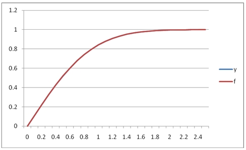
We can see that in this range, [0, 2.5] the fit between the y-values and the f-values (ERF(x) in this case) is quite good. Since POLYVAL creates an approximating polynomial, it is not bound by minima and maxima of x-y pairs. In this example, we will graph the results this SQL, which will using the approximating polynomial from the [0, 2.5] interval on the interval [0, 6].
SET NOCOUNT ON;

SELECT SeriesValue as x
,westclintech.wct.ERF(SeriesValue) as y
INTO #erf
FROM wct.SeriesFloat(0,2.5,0.1,NULL,NULL);

SELECT a.seriesvalue as x
,wct.POLYVAL(e.x, e.y, 6, seriesvalue) as POLYVAL
FROM wct.SERIESFLOAT(0.0,6.0,0.1,NULL,NULL) a
,#erf E
GROUP BY seriesvalue;

DROP TABLE #erf;
This produces the following graph.
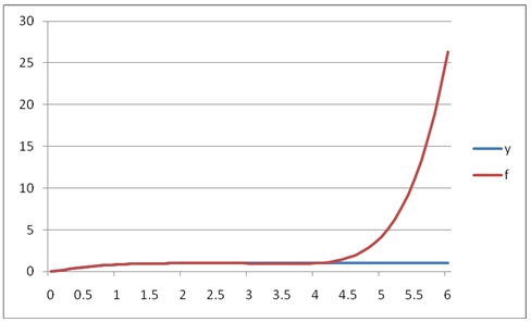
As you can see, the polynomial approximation quickly diverges from the function in the region above 2.5. Let's look at how POLYVAL works with dates. In this example we will look at some interest rate values over a time-horizon and calculate the 3rd degree polynomial approximation. The x-values are dates and the y-values are the decimal values of the interest rate (.01 = 1%).
SET NOCOUNT ON;
SELECT cast(x as datetime) as x,
       y
INTO #a
FROM
(
    VALUES
        ('2012-Apr-30', 0.0028),
        ('2013-Apr-30', 0.0056),
        ('2014-Apr-30', 0.0085),
        ('2016-Apr-30', 0.0164),
        ('2018-Apr-30', 0.0235),
        ('2021-Apr-30', 0.0299),
        ('2031-Apr-30', 0.0382),
        ('2041-Apr-30', 0.0406)
) m (x, y);
SELECT wct.POLYVAL(cast(x as float), y, 3, cast(Cast('2012-Oct-31' as datetime)
          as float)) as POLYVAL
from #a;
DROP TABLE #a;
This produces the following result.
| POLYVAL |
|---|
| 0.00378351662681808 |
In this example we will use POLYVAL, the SeriesInt function and the EOMONTH function from XLeratorDB/financial to calculate the rates for each year from 1 through 30 out to 4 decimal places.
SET NOCOUNT ON;
SELECT cast(x as datetime) as x,
       y
INTO #a
FROM
(
    VALUES
        ('2012-Apr-30', 0.0028),
        ('2013-Apr-30', 0.0056),
        ('2014-Apr-30', 0.0085),
        ('2016-Apr-30', 0.0164),
        ('2018-Apr-30', 0.0235),
        ('2021-Apr-30', 0.0299),
        ('2031-Apr-30', 0.0382),
        ('2041-Apr-30', 0.0406)
) m (x, y);
SELECT convert(varchar, wct.EOMONTH('04/30/2011', SeriesValue), 106) as [MATURITY
          DATE],
       ROUND(wct.POLYVAL(cast(x as float), y, 3, cast(wct.EOMONTH('04/30/2011',
                 SeriesValue) as float)), 4) as [INTEREST RATE]
from #a,
     wct.SeriesInt(12, 360, 12, NULL, NULL)
GROUP BY wct.EOMONTH('04/30/2011', SeriesValue);
DROP TABLE #a;
This produces the following result.
| MATURITY DATE | INTEREST RATE |
|---|---|
| 30 Apr 2012 | 0.0015 |
| 30 Apr 2013 | 0.0059 |
| 30 Apr 2014 | 0.0099 |
| 30 Apr 2015 | 0.0136 |
| 30 Apr 2016 | 0.017 |
| 30 Apr 2017 | 0.02 |
| 30 Apr 2018 | 0.0228 |
| 30 Apr 2019 | 0.0252 |
| 30 Apr 2020 | 0.0274 |
| 30 Apr 2021 | 0.0293 |
| 30 Apr 2022 | 0.031 |
| 30 Apr 2023 | 0.0325 |
| 30 Apr 2024 | 0.0338 |
| 30 Apr 2025 | 0.0349 |
| 30 Apr 2026 | 0.0358 |
| 30 Apr 2027 | 0.0366 |
| 30 Apr 2028 | 0.0373 |
| 30 Apr 2029 | 0.0378 |
| 30 Apr 2030 | 0.0382 |
| 30 Apr 2031 | 0.0385 |
| 30 Apr 2032 | 0.0388 |
| 30 Apr 2033 | 0.039 |
| 30 Apr 2034 | 0.0391 |
| 30 Apr 2035 | 0.0393 |
| 30 Apr 2036 | 0.0394 |
| 30 Apr 2037 | 0.0395 |
| 30 Apr 2038 | 0.0397 |
| 30 Apr 2039 | 0.0399 |
| 30 Apr 2040 | 0.0402 |
| 30 Apr 2041 | 0.0405 |